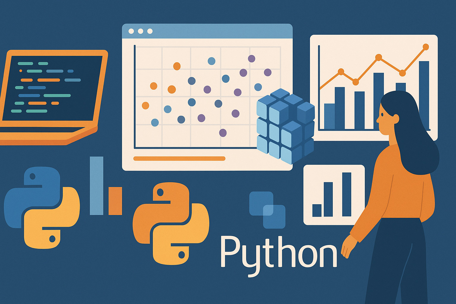
Using Python as the Foundation of Data Analysis and Modeling
Data science is rapidly becoming a part of daily life in organizations, businesses, and academia. Behind visualizations, predictions, and automated decisions are tools that help us make sense of large datasets. One of the most popular and effective ways to do this is through Python and its libraries—NumPy and Pandas.
When working with data, you need tools that are fast, flexible, and easy to understand. That’s exactly what NumPy and Pandas provide. You don’t have to build everything from scratch—these libraries offer built-in functions for data analysis, format transformation, and even complex computations like statistical analysis.
Python’s widespread use in data science isn’t just due to its clean syntax, but also its large community and rich ecosystem of libraries. With NumPy for numerical operations and Pandas for structured data, each project becomes more organized, the results clearer, and the turnaround time faster.
Understanding NumPy and Why It Matters
NumPy is a foundational library for numerical computing in Python. It’s often the first step for anyone entering data science. Its core feature is the ndarray, a highly efficient data structure for high-performance arrays.
Unlike native Python lists, NumPy arrays are faster and more memory-efficient. It includes built-in mathematical operations that apply to entire arrays without the need for loops. So, even when processing millions of data points, performance remains smooth.
Beyond speed, NumPy also offers functions for linear algebra, statistics, random sampling, and Fourier transforms—all within a consistent framework that’s easy to follow and integrates well with other tools like Scikit-learn or Matplotlib.
Start Manipulating Arrays with NumPy
Once you have data, the next step is to manipulate it for analysis. With NumPy, you can slice arrays, transform them, broadcast operations, or reshape arrays using functions like reshape() or transpose(). From simple 1D arrays to complex multi-dimensional matrices—NumPy handles it all.
For example, if you have an array of daily product prices, you can quickly calculate the average, variance, or maximum value using np.mean(), np.var(), and np.max(). No need for nested loops or long formulas—just one line of code does the job.
These operations are essential when working with time series, image data, or scientific datasets. NumPy’s simple syntax and fast computation make it an everyday part of a data scientist’s workflow.
Moving from NumPy to Pandas for Structured Data
While NumPy excels with numerical arrays, Pandas is better suited for labeled data—like spreadsheets, CSV files, or SQL tables. This is where Pandas comes into play. It has two main data structures: Series and DataFrame.
A DataFrame is like an Excel table with rows, columns, and headers. With a single command like pd.read_csv(), you can load data and immediately begin filtering, sorting, and aggregating. Tasks that are typically manual in spreadsheets can be automated with Pandas.
Combined, NumPy and Pandas offer speed and structure. Use NumPy for high-speed computation and Pandas for better readability and data access. They are often used together in almost all modern data workflows in Python.
Data Cleaning with Pandas: A Daily Task
Before you can visualize or model data, you must clean the raw data. This is where Pandas shines. Most raw datasets come with missing values, inconsistent entries, or incorrect data types. Pandas helps fix this with just a few lines of code.
For example, use dropna() to remove rows with missing values, or fillna(df.mean()) to fill gaps with the average. Changing column types, merging tables, or filtering rows can all be done with function chains.
While not the most glamorous part of data science, cleaning is the foundation of accurate analysis. Pandas makes this process faster and less error-prone. Mastering it significantly boosts your effectiveness as a data analyst.
Analyzing Data with Aggregation and Grouping
Once your data is clean, the next step is analysis. Pandas offers built-in methods like groupby(), agg(), and pivot_table() for combining, breaking down, or summarizing data across categories.
For instance, use df.groupby(‘Region’)[‘Sales’].mean() to get average sales per region in one line—a task that would take several minutes in a spreadsheet. Even better, the code is reusable and reproducible.
This method of aggregation reveals clear insights. For more complex summaries, you can combine multiple functions in agg() using dictionaries. Patterns, outliers, and trends become visible even before visualization.
Visualization with Pandas and Matplotlib
After analysis, visualizing the results helps communicate them better. Pandas has built-in support for Matplotlib, allowing you to create bar charts, line graphs, histograms, and more using the .plot() method on DataFrames or Series.
Visualization isn’t just for aesthetics—it reveals patterns hidden in raw numbers. In a sales dataset, you might miss seasonality at a glance, but a line chart can immediately show peak months.
For more detailed visuals, you can use Seaborn or Plotly. However, Pandas plotting is usually sufficient for most projects. Simplicity is key—just one command can give you the chart you need.
Using Pandas for Time Series Analysis
One of Pandas’ strengths is its support for time series data. If your data includes dates—like daily transactions, stock prices, or sensor readings—it’s easy to analyze with datetime indexing, resampling, and rolling windows.
With pd.to_datetime(), you can convert a column into a datetime format. Once indexed, use resample() to calculate monthly averages or weekly totals—perfect for time-based analyses.
The rolling() method helps compute moving averages or cumulative sums. This is especially important in finance and forecasting. With just a few lines of code, you can gain deep insights from simple date-based data.
Combining Data from Multiple Sources
Most real-world datasets don’t come from a single file. You might have data from CSVs, APIs, Excel sheets, or databases. In Pandas, you can easily merge them using merge(), concat(), or join().
For example, merge sales data with customer data using a common ID, or combine two similarly structured DataFrames with concat() to build a larger dataset.
This data integration enables holistic analysis. You’re not limited to what’s in one file. Integration in Pandas is simple but powerful—and since it’s still within Python, you can extend it to APIs or real-time streaming sources.
Easier Analysis with NumPy and Pandas
NumPy and Pandas provide a solid foundation for data science in Python. They’re not just tools—they’re essential parts of the data analysis ecosystem. NumPy gives you a fast, efficient numerical engine; Pandas gives you a flexible, powerful structure for managing structured data.
Together, they simplify everything from loading and cleaning data to analysis and visualization. You don’t need long scripts to get meaningful results. And because they’re open-source with strong communities, there’s always something new to learn—updates, plugins, or best practices.
For those serious about getting into data science with Python, mastering NumPy and Pandas is a strong starting point. Once you’re familiar with them, transitioning to more advanced libraries like Scikit-learn, TensorFlow, or Statsmodels becomes much easier.